Best practices for HEC-RAS 2D modeling with AutoCAD Civil 3D

I've had enough experience now using AutoCAD Civil 3D and HEC-RAS for 2D flow modeling in Maricopa County Arizona to share a list of best practices. It's only a small beginning, but it's something. Enjoy.

HEC-RAS 2D Modeling With AutoCAD Civil 3D - Best Practices

Terrain

Feel free to use high density DEM export

While AutoCAD is slow to handle and export high density models, HEC-RAS does not seem to choke on them. I have used 1-foot density on a terrain model of about 2 square miles, and HEC-RAS handled it well.

Export from AutoCAD with Average Elevation

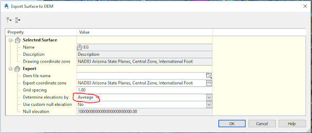
When you Export Surface to DEM, choose Determine elevations by Average rather than Sample surface at grid point. Some smoothing, while slower and not perfect, is better (more predictable and uniform) than randomly capturing varying approaches to anomalies or sharp edges in the terrain.

Determine elevations by Average rather than Sample surface at grid point

Organize your terrain work flow

If you have a design that affects your terrain, the cycle of terrain tweaks can be very time consuming (expensive). Keep a written list of pending terrain tweaks to minimize the number and frequency of terrain tweak cycles.

Roughness

If you have more than one roughness in a 2D area, you need to use a Land Use model like this.

Use ADE commands to attach data to roughness area polylines

The ADEDEFDATA and ADEATTACHDATA commands are an easy way to attach Land Use Type names to roughness area polylines for transfer from AutoCAD to HEC-RAS. See more below.

Organize your roughness model in AutoCAD

The screen shot below shows the AutoCAD layer for all the roughness region polylines (top lasso). It also shows the ADEDEFDATA data "table" definition for the Land Use Type names you will send to HEC-RAS for translation to roughnesses.

Use Land Use Type names rather than roughness values in AutoCAD

After you use ADEATTACHDATA to attach the HEC-RAS-LAND data table to your roughness region polylines, at the bottom of Properties, assign a roughness type name (Obstruction, Pavement, Shotcrete, etc), to each polyline. You will tell HEC-RAS how to translate each type into a roughness. You can leave the dominant roughness undelineated to let it use the default roughness for the 2D area in HEC-RAS.

Use high roughness regions to add obstructions to the terrain

Buildings and other massive obstructions can be modeled as regions of high roughness. Be aware that this may be inaccurate in that it allows storage inside the obstruction. If the obstruction models are critical to downstream hydrographs (such as if you have a steeply rising hydrograph with a sharp peak) it may be better to modify the terrain.

In HEC-RAS, use a high density land use layer grid

Use a density as high as your terrain density for the rendering of your roughness regions in HEC-RAS.

HEC-RAS 2D Area Grid

Consider expected WSE slope and desired WSE density

The biggest limitation of the underlying HEC-RAS hydraulic approach for 2D modeling is that all grid cells/faces have level water surfaces, and this would not be an easy simplification to improve on. For steep water surface slopes, this may be the single factor that pushes your cell spacing smaller. Do an occasional calculation in your head of the anticipated WSE change from one cell to the next and keep in mind the discontinuities that are at play at cell faces and corners due to the level cell face water surfaces.

Start with low density (big cells)

2D area density is a decision that makes a huge difference in your time investment. You control the model run time ranging from seconds to hours starting with the grid density you choose. Do not make the mistake of starting small. Start large. The good news is that in spite of the level WSE limitation, the underlying hydraulics of HEC-RAS are impressive in that they calculate a true 1D terrain cross section at each cell face. This means that the terrain density of your model is NOT limited by your 2D cell grid density. In other words, if your terrain has 0.3-meter density, that density is accurately modeled EVEN IF your 2D grid spacing is 10 meters or more. Trust me. Start big. Try it. You will like the results.

Supplement 2D cell grid with 2D Area Break Lines

But each cell face is just a dumb 1D model that will calculate split flow inappropriately just like any 1D model cross section (These are areas where you would have perhaps received the 1D warning: Divided flow at RS XX.XXX). Part of your model improvement/discovery cycle will be to add 2D area breaklines at key drainage divides and weirs to allow the proper calculation of divided flow splits.

Wherever you see flow violating drainage divides by magically flowing through them, you need to add 2D Area Break Lines. They are much more effective and efficient (for your project schedule and budget) than reducing your 2D Area cell spacing. They are your friends.

The more models I do and the more 2D Area Break Lines I add, the more I tend to leave their cell spacing at the grid defaults. See calculation time step discussion.

Resolve grid errors by small tweaks

When you are having trouble building the grid without errors, resolve the errors with minor adjustments to the 2D Area boundary and 2D Area Break Lines (Move points, Add point, Remove points) or cell spacing (such as changing spacing from 30 to 31 or 29).

Calculation

Grid cell spacing that is too small does not only hurt you by proliferating grid cells and faces inversely proportional to the square of cell spacing. It also reduces the time delay between faces, causing you to have to reduce your computation time step. So you want to keep in mind that your modeling cycle time increases approximately proportional to grid cell spacing cubed! Where a cell spacing of 8 meters (26 feet) might take 1 minute to compute, a cell spacing of 2 meters (7 feet) might take 1 hour.

Unsteady Flow Analysis

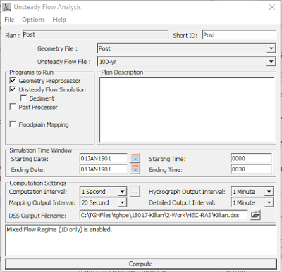
The first goal in unsteady flow analysis is to get your model to run. The second goal is to get it to run with acceptable WSE errors. Here are some screen shots showing settings for a smaller project with 10-foot cell spacing where cycle time was not as critical as for a larger model.

Unsteady Flow Analysis settings for a small project with 10-foot cell spacing

Unsteady Computation Options and Tolerances

In the above, if velocities were expected to be lower, Computation Interval could probably be increased.

Start big and reduce until it runs

Absent any other information, guess the minimum wave diffusion time between cell faces (or distance divided by velocity) and start with that as your Computation Interval.

Unsteady Flow Data

HEC-DSS

HEC-RAS reads hydrographs from HEC-DSS files. I export those from HEC-1 (probably can be done from HEC-HMS too).

Tips

Terrain

• As of version 5.0.7, you sometimes have to exit HEC-RAS to get a RAS Mapper terrain update to reflect in Geometry Editor.
• Warning: as of version 5.0.7, RAS Mapper saves all changes automatically.

Projection

• You can use a scaled (ground distances) projection. But if you do, you can't use any Web Imagery, since as of version 5.0.7, Web Imagery does not scale.